Introduction to NLP
We will cover practical NLP:
- how to process text
- how to do useful things with it
... we will not cover theoretical NLP:
- grammars, syntax, linguistic models
- (sorry Noam)
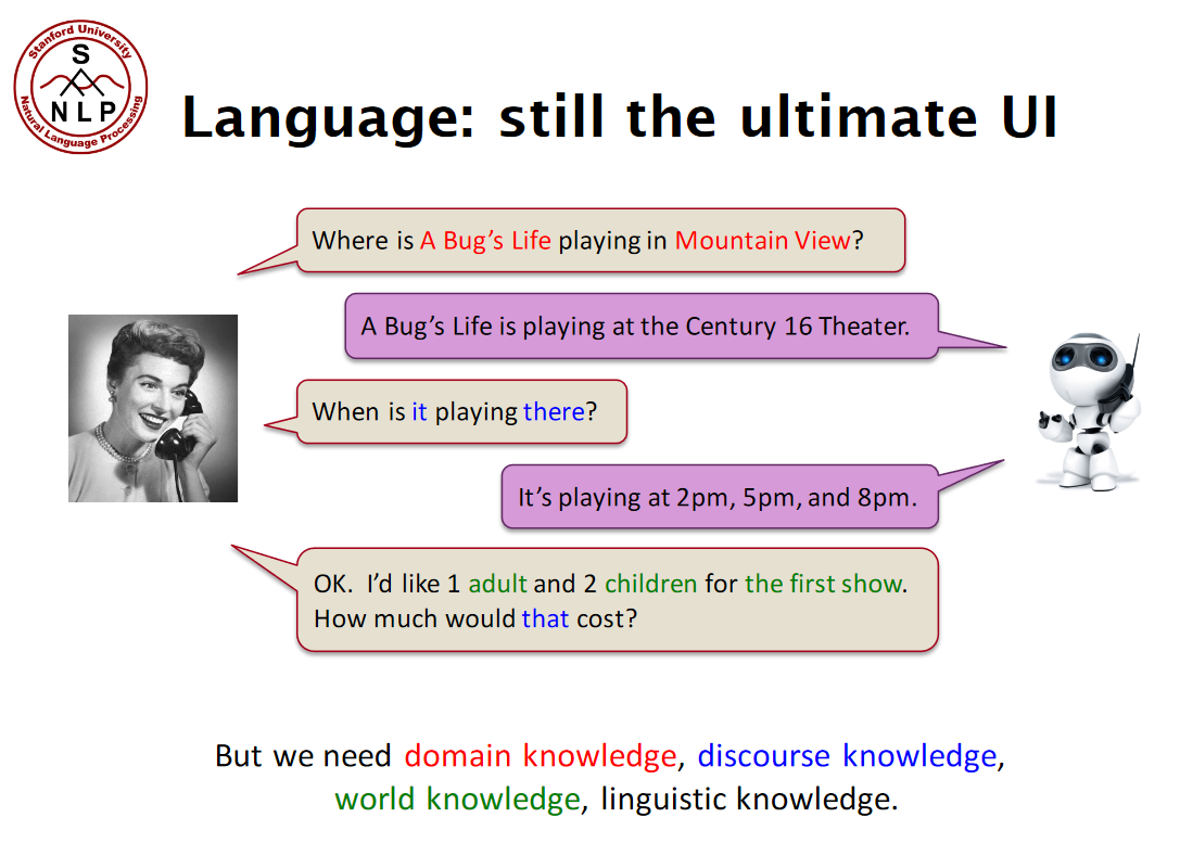
Why is NLP hard?


Why is NLP hard?
- ambiguous
- complex
- context dependent
- requires prior knowledge
- requires a world model
- is used for interaction with people (amusing, insulting)
Famous NLP successes
Words as data
Let's start with some very short reviews, and our goal is to classify whether they are positive (1) or negative (0) in terms of sentiment, i.e. whether someone liked the movie or not.
sentences = [
    'We had a good time.',
    'This was a good-looking place.',
    'A once in a lifetime experience.',
    'Horrible.',
    'One of the worst experiences of my life.',
    "Everything went terribly, I'll never return."
]
y = [1, 1, 1, 0, 0, 0]
Create a feature matrix
- We need to transform
sentenceinto a matrix of features (X) - < w1, w2, ..., wM > -> xi
- How would you do this?
A silly approach
We can memorize the sentences, and output the known answer.
# create a dictionary which maps each sentence to a known outcome
model = {sentences[i]: y[i] for i in range(len(sentences))}
print('Model')
for sentence, target in model.items():
    print(f'  {sentence}: {target}')


# see how often our model is correct
print('\nPerformance')
match = [model[sentence] == y[i] for i, sentence in enumerate(sentences)]
print(f'{sum(match) / len(sentences):3.1%} accuracy.')
Model
  We had a good time.: 1
  This was a good-looking place.: 1
  A once in a lifetime experience.: 1
  Horrible.: 0
  One of the worst experiences of my life.: 0
  Everything went terribly, I'll never return.: 0

Performance
100.0% accuracy.
What if we try a new sentence?
sentence = ""
target = 0
sentences_test = [
    'This was fun!',
    'Abysmal service.'
]
y_test = [1, 0]

try:
    match = [model[sentence] == y[i] for i, sentence in enumerate(sentences_test)]
    print(f'{sum(match) / len(sentences_test):3.1%} accuracy.')
except KeyError as err:
    print(f'Sentence not found in model!')
Sentence not found in model!
Here is the traceback for the error we would have had without the try/except block:
---------------------------------------------------------------------------
KeyError                                  Traceback (most recent call last)
<ipython-input-5-1d2b9ac74b7f> in <module>
----> 1 match = [model[sentence] == y[i] for i, sentence in enumerate(sentences_test)]
      2 print(f'{sum(match) / len(sentences_test):3.1%} accuracy.')

<ipython-input-5-1d2b9ac74b7f> in <listcomp>(.0)
----> 1 match = [model[sentence] == y[i] for i, sentence in enumerate(sentences_test)]
      2 print(f'{sum(match) / len(sentences_test):3.1%} accuracy.')

KeyError: 'This was fun!'
Create a feature matrix
- We need to transform a
sentenceinto a matrix of features (X). - We can represent a
sentenceas a collection of symbols s
[s1, s2, ..., sM] ---> [x1, x2, ..., xD]
Note D (length of x) != M (number of symbols in the sentence).
- How would you do this?
A slightly less silly approach
One feature for every letter in the alphabet
| s1 | s2 | s3 | s4 | to | x1 | x2 | ||
|---|---|---|---|---|---|---|---|---|
| d | i | p | 0 | 1 | ||||
| c | a | t | 0 | 0 | ||||
| h | i | 1 | 0 | |||||
| s | h | i | p | 1 | 1 |
alphabet='abcdefghijklmnopqrstuvwxyz'
def prepare_data(sentences, alphabet=alphabet):
    return [[int(a in sentence) for a in alphabet] for sentence in sentences]

X = prepare_data(sentences)
# visualize the data with the sentence
print(alphabet)
for i, sentence_vector in enumerate(X):
    print(''.join([str(c) for c in sentence_vector]), end=' ')
    print(sentences[i])
abcdefghijklmnopqrstuvwxyz
10011011100010100001000000 We had a good time.
10111011101101110010001000 This was a good-looking place.
10101100100111110101000100 A once in a lifetime experience.
01001000100100100100000000 Horrible.
00101101100111110111001110 One of the worst experiences of my life.
01001011100101000101111010 Everything went terribly, I'll never return.
Train the model
mdl = tree.DecisionTreeClassifier(max_depth=3)

# fit the model to the data - trying to predict y from X
mdl = mdl.fit(X, y)
Try our model on new data
X_test = prepare_data(sentences_test)
pred_test = mdl.predict(X_test)

match = [pred_test[i] == y_test[i] for i, sentence in enumerate(sentences_test)]
print(f'{sum(match) / len(sentences_test):3.1%} accuracy.')
print([(pred_test[i], sentence) for i, sentence in enumerate(sentences_test)])
50.0% accuracy.
[(1, 'This was fun!'), (1, 'Abysmal service.')]
That's... bad. What happened?
Visualize the trained model
graph = create_graph(mdl, feature_names=list(alphabet))
Image(graph.create_png())

# print out the training set with the letter "a" highlighted in each sentence
for i, sentence in enumerate(sentences):
    sentence = ''.join([f"\033[1m\033[91m{c}\033[0m"  if c == 'a' else c for c in sentence])
    print(f'{sentence}: {y[i]}')
We had a good time.: 1
This was a good-looking place.: 1
A once in a lifetime experience.: 1
Horrible.: 0
One of the worst experiences of my life.: 0
Everything went terribly, I'll never return.: 0
NLP has many levels
- Symbol/Character
- Lexeme
- Word
- Sentence
- Paragraph, Document, Corpus, ...
NLP has many levels
- ~Symbol/Character~ - too low level (on its own!)
- ~Lexeme~ - we don't know what this means
- Word
- ~Sentence~ - too high level
- ~Paragraph, Document, Corpus, ...~ - same issue as sentences
Words as data
- Our "alphabet" becomes all the words we've seen
- Before:
alphabet = ['a', 'b', 'c', 'd', ...] - Now:
alphabet = ['good', 'bad', 'movie', ...]
- Before:
import itertools

# get all the unique words in the sentences, splitting by spaces
alphabet = sorted(list(set(
    [word for sentence in sentences
     for word in sentence.split(' ')]
)))
print(alphabet)
['A', 'Everything', 'Horrible.', "I'll", 'One', 'This', 'We', 'a', 'experience.', 'experiences', 'good', 'good-looking', 'had', 'in', 'life.', 'lifetime', 'my', 'never', 'of', 'once', 'place.', 'return.', 'terribly,', 'the', 'time.', 'was', 'went', 'worst']
The above list.. isn't great.
- punctuation included in words
- "experience" and "experiences" separate
- "A" and "a" are different
- "good-looking" vs "good"
Hrm, that's annoying.
This should be the motto for NLP.
Words as data
- Focus on the word "good-looking".
- Should we split this into two words, "good" and "looking"?
- What about
I'll? Strictly speaking, it's two words:Iandwill.
Tokenization
- In NLP, we don't work with "words", we work with "tokens"
- Tokens are groups of symbols with some semantic meaning
- Tokenization is the process of converting text into individual tokens
Tokenizers
Trying it out
We'll work with spaCy's tokenizer.
import spacy
# load an English spacy model we have already downloaded
nlp = spacy.load("en_core_web_sm")
Trying it out
for sentence in sentences:
    doc = nlp(sentence)
    print(sentence, end=': ')
    print([token for token in doc])
We had a good time.: [We, had, a, good, time, .]
This was a good-looking place.: [This, was, a, good, -, looking, place, .]
A once in a lifetime experience.: [A, once, in, a, lifetime, experience, .]
Horrible.: [Horrible, .]
One of the worst experiences of my life.: [One, of, the, worst, experiences, of, my, life, .]
Everything went terribly, I'll never return.: [Everything, went, terribly, ,, I, 'll, never, return, .]
Trying it out
We can try other sentences to explore the tokenizer's quirks.
sentence = "To be or not to be; that is the question. Or at least it was Hamlet's question."
doc = nlp(sentence)
print([token for token in doc])
[To, be, or, not, to, be, ;, that, is, the, question, ., Or, at, least, it, was, Hamlet, 's, question, .]
Rather than continue with the dummy dataset, let's get our hands on some real data.
IMDb
A large dataset from the Internet Movie Database (IMDb) was curated by researchers [1].
- 50,000 reviews of movies on IMDB
- 25,000 positive reviews (>=7), 25,000 negative reviews (<=4)
- Commonly used for sentiment classification; i.e. is this review positive (great movie!) or negative (awful movie!)
[1] Maas A, Daly RE, Pham PT, Huang D, Ng AY, Potts C. Learning word vectors for sentiment analysis. In Proceedings of the 49th annual meeting of the association for computational linguistics: Human language technologies 2011 Jun (pp. 142-150).
def load_data(path):
    # initialize a dictionary (key-value store) for our corpus
    corpus = {}

    # for each file in the given folder path
    files = os.listdir(path)
    for fn in tqdm(files):
        filename = path / fn
        # open the file and read the text
        with open(filename, 'r') as fp:
            text = ''.join(fp.readlines())

        # put the text into the dictionary keyed by the filename
        # we can later access text data by indexing this dictionary
        # e.g. corpus["10_9"]
        corpus[filename.stem] = text

    return corpus

print('Loading positive documents (training set).')
pos = load_data(Path('aclImdb/train/pos'))
print('Loading negative documents (training set).')
neg = load_data(Path('aclImdb/train/neg'))

print('Loading positive documents (test set).')
pos_test = load_data(Path('aclImdb/test/pos'))
print('Loading negative documents (test set).')
neg_test = load_data(Path('aclImdb/test/neg'))

def get_numpy_arrays(pos, neg):
    # create numpy arrays of the datasets
    # these are more natively usable by ML libraries
    X_pos = np.array(list(pos.values()))
    X_neg = np.array(list(neg.values()))
    X = np.hstack([X_pos, X_neg])
    n_pos, n_neg = X_pos.shape[0], X_neg.shape[0]
    y = np.concatenate([np.ones(n_pos), np.zeros(n_neg)])
    return X, y

# only use ~1000 examples for speed
X_train, y_train = get_numpy_arrays(
    {k: v for k, v in pos.items() if k.startswith('2')},
    {k: v for k, v in neg.items() if k.startswith('2')}
)
X_test, y_test = get_numpy_arrays(
    {k: v for k, v in pos_test.items() if k.startswith('2')},
    {k: v for k, v in neg_test.items() if k.startswith('2')}
)
Loading positive documents (training set).
Loading negative documents (training set).
Loading positive documents (test set).
Loading negative documents (test set).
Example review - Stanley and Iris

Example review - Stanley and Iris
review = pos['10_9']
print(review)
I'm a male, not given to women's movies, but this is really a well done special story. I have no personal love for Jane Fonda as a person but she does one Hell of a fine job, while DeNiro is his usual superb self. Everything is so well done: acting, directing, visuals, settings, photography, casting. If you can enjoy a story of real people and real love - this is a winner.
Redo our character example with sklearn
With the mock dataset, we manually created the feature matrices with characters as features.
Now we'll use scikit-learn for modelling. Read more about the components of scikit-learn:
- Pipeline - compose operations commonly applied in ML
- CountVectorizer - convert text into features
- User Guide on text feature extraction - a good intro into using scikit-learn for NLP
- Decision Trees - decision trees are a simple ML model - colab tutorial on decision trees and more complex tree based models (e.g. xgboost)
Build the model
We'll focus on changing the arguments to Pipeline - and the utility functions defined above will use the pipeline to train a model using the training data and apply it to the test data.
pipe = Pipeline([('vectorizer', CountVectorizer(
                    analyzer='char',
                    binary=True)
                 ),
                 ('classifier', tree.DecisionTreeClassifier(max_depth=3))])

# pipeline will be updated in-place!
pred = train_pipe_and_predict(pipe, X_train, y_train, X_test)

# Now that we have predictions for the test set (`pred`), we can calculate the performance of our model on a held out set.
print_results(y_test, pred)
Building model.
Getting test predictions.
Accuracy: 57.8%
Precision: 56.2%
Recall: 71.0%
Visualize the model
# grab the vectorizer / classifier to make a figure of the model
vectorizer = pipe.named_steps['vectorizer']
classifier = pipe.named_steps['classifier']

graph = create_graph(classifier, feature_names=vectorizer.get_feature_names())
Image(graph.create_png())

Note that our CountVectorizer class has added symbols beyond the alphabet.
print([c for c in sorted(list(vectorizer.vocabulary_.keys()))])
['\t', '\x10', ' ', '!', '"', '#', '$', '%', '&', "'", '(', ')', '*', '+', ',', '-', '.', '/', '0', '1', '2', '3', '4', '5', '6', '7', '8', '9', ':', ';', '<', '=', '>', '?', '@', '[', '\\', ']', '^', '_', '`', 'a', 'b', 'c', 'd', 'e', 'f', 'g', 'h', 'i', 'j', 'k', 'l', 'm', 'n', 'o', 'p', 'q', 'r', 's', 't', 'u', 'v', 'w', 'x', 'y', 'z', '{', '|', '}', '~', '\x80', '\x85', '\x91', '\x96', '\x97', '¡', '£', '¨', '´', '½', 'à', 'á', 'ã', 'ä', 'ç', 'è', 'é', 'í', 'î', 'ï', 'ñ', 'ó', 'ô', 'ö', 'ú', 'û', 'ü', '’', '“', '”']
Compare approaches
- Binary character presence: 57.8%.
Count the characters rather than present/absent
In our above pipeline, we specified binary=True. From the scikit-learn docs on CountVectorizer:
binary bool, default=False
If True, all non zero counts are set to 1. This is useful for discrete probabilistic models that model binary events rather than integer counts.
This creates what we had before - a feature matrix of 1s and 0s. As the name implies, CountVectorizer is able to return a matrix of counts for how often a character appears. We can see the impact of changing this below.
pipe = Pipeline([('vectorizer', CountVectorizer(
                    analyzer='char',
                    binary=False)
                 ),
                 ('classifier', tree.DecisionTreeClassifier(max_depth=3))])

# pipeline will be updated in-place!
pred = train_pipe_and_predict(pipe, X_train, y_train, X_test)

# Now that we have predictions for the test set (`pred`), we can calculate the performance of our model on a held out set.
print_results(y_test, pred)
Building model.
Getting test predictions.
Accuracy: 55.4%
Precision: 53.6%
Recall: 81.2%
Compare approaches
- Character presence: 57.8%.
- Character counts: 55.4%.
Recap
- We tried to classify some dummy text using the presence of letters
- It did not go well
- We are going to try using the presence of words
- We hope it will go better!
Tokenize the review
doc = nlp(review)
print([token for token in doc])
[I, 'm, a, male, ,, not, given, to, women, 's, movies, ,, but, this, is, really, a, well, done, special, story, ., I, have, no, personal, love, for, Jane, Fonda, as, a, person, but, she, does, one, Hell, of, a, fine, job, ,, while, DeNiro, is, his, usual, superb, self, ., Everything, is, so, well, done, :, acting, ,, directing, ,, visuals, ,, settings, ,, photography, ,, casting, ., If, you, can, enjoy, a, story, of, real, people, and, real, love, -, this, is, a, winner, .]
'mand'sare given their own token- punctuation marks are individual tokens
- whitespaces are individual tokens
As you can see, tokens do not have to be words!
... how do we turn this into X?
Creating the feature matrix
- Recall when we used the alphabet
- Each column was a letter
- Each row was our sentence (now review)
X[i,j] == 1-> letter is in the documentX[i,j] == 0-> letter is not in the document
- We are using tokens instead of letters
- Advantage: we think words will be a better representation of text meaning (compared to letters)
- Disadvantage: we now need to create an "alphabet" for words, i.e. the vocabulary
Vocabulary
- The set of tokens we choose is our vocabulary.
- Most vocabularies consist of the most common tokens.
"You will know 90% of the words in a book after the first 20 pages, so the rest of it will be easier to read.."
 |
 |
 |


def spacy_tokenizer(text):
    return [token.text for token in nlp.tokenizer(text)]
pipe = Pipeline([('vectorizer', CountVectorizer(tokenizer=spacy_tokenizer, max_features=10, binary=True)),
                 ('classifier', tree.DecisionTreeClassifier(max_depth=3))])

# pipeline will be updated in-place!
pred = train_pipe_and_predict(pipe, X_train, y_train, X_test)

# Model Accuracy
print_results(y_test, pred)
Building model.
Getting test predictions.
Accuracy: 49.5%
Precision: 49.7%
Recall: 90.9%
We now have 50% accuracy - no better than chance - yikes! What happened?
Well, we did select only the top 10 tokens (max_features=10). What do you think the top 10 tokens are in the IMDb dataset?
from collections import Counter

token_freq = Counter()

for corpus in [pos, neg]:
    for text in tqdm(corpus.values(), total=len(corpus)):
        # only call the tokenizer for speed purposes
        doc = nlp.tokenizer(text)

        for token in doc:
            # use 'orth', the integer version of the string
            # will convert back to string version later
            token_freq[token.orth] += 1

# convert back to string
token_freq = Counter({nlp.vocab.strings[k]: v for k, v in token_freq.items()})
The most popular word in each state
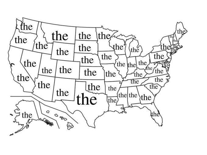
token_freq.most_common(10)
[('the', 289838),
 (',', 275296),
 ('.', 236702),
 ('and', 156484),
 ('a', 156282),
 ('of', 144056),
 ('to', 133886),
 ('is', 109095),
 ('in', 87676),
 ('I', 77546)]
text = pos['10_9']
print(text, end='\n\n')
freq = vectorizer.transform([text])[0].toarray()
features = vectorizer.get_feature_names()
for i, feat in enumerate(features):
    print(f'{feat:10s} {freq[0][i]:3d}')
I'm a male, not given to women's movies, but this is really a well done special story. I have no personal love for Jane Fonda as a person but she does one Hell of a fine job, while DeNiro is his usual superb self. Everything is so well done: acting, directing, visuals, settings, photography, casting. If you can enjoy a story of real people and real love - this is a winner.
0
0
1
! 0
" 0
# 0
$ 0
% 0
& 0
' 1
( 0
) 0
* 0
+ 0
, 1
- 1
. 1
/ 0
0 0
1 0
2 0
3 0
4 0
5 0
6 0
7 0
8 0
9 0
: 1
; 0
< 0
= 0
> 0
? 0
@ 0
[ 0
\ 0
] 0
^ 0
_ 0
` 0
a 1
b 1
c 1
d 1
e 1
f 1
g 1
h 1
i 1
j 1
k 0
l 1
m 1
n 1
o 1
p 1
q 0
r 1
s 1
t 1
u 1
v 1
w 1
x 0
y 1
z 0
{ 0
| 0
} 0
~ 0
0
0
0
0
0
¡ 0
£ 0
¨ 0
´ 0
½ 0
à 0
á 0
ã 0
ä 0
ç 0
è 0
é 0
í 0
î 0
ï 0
ñ 0
ó 0
ô 0
ö 0
ú 0
û 0
ü 0
’ 0
“ 0
” 0
Stop words
- The tokens "the", ",", etc have little meaning on their own
- We call these "stop words".
- Stop word removal: delete these words from the text.
def spacy_tokenizer(text):
    return [token.text for token in nlp.tokenizer(text) if not token.is_punct and not token.is_stop]
Note: There is no universal list of stop words! Everyone has their own flavor, including spacy.
# train the model with our updated spacy_tokenizer, which removes stop words
pipe = Pipeline([('vectorizer', CountVectorizer(tokenizer=spacy_tokenizer, max_features=10, binary=True)),
                 ('classifier', tree.DecisionTreeClassifier(max_depth=3))])

pred = train_pipe_and_predict(pipe, X_train, y_train, X_test)

print_results(y_test, pred)
Building model.
Getting test predictions.
Accuracy: 59.7%
Precision: 58.8%
Recall: 64.4%
vectorizer = pipe.named_steps['vectorizer']
classifier = pipe.named_steps['classifier']

graph = create_graph(classifier, feature_names=vectorizer.get_feature_names())
Image(graph.create_png())

text = pos['10_9']
introspect_text(pipe, text)
I'm a male, not given to women's movies, but this is really a well done special story. I have no personal love for Jane Fonda as a person but she does one Hell of a fine job, while DeNiro is his usual superb self. Everything is so well done: acting, directing, visuals, settings, photography, casting. If you can enjoy a story of real people and real love - this is a winner.

Prediction: POSITIVE.
/><br        0
film         0
good         0
great        0
like         0
movie        0
people       1
story        1
time         0
way          0
Compare approaches
- Character binary: 57.8%.
- Character counts: 55.4%.
- Token binary: 49.5%.
- Token stop word removal binary: 59.7%.
Should you always remove stop words?

Should you always remove stop-words?
Well - obviously the answer is no. But why was it helpful above?
Answer: We had already destroyed our document structure.
- The act of counting words removes any semblence of word order
- Stop words frequently only have meaning when retaining text structure
- Most obvious if you think about punctuation as stop words
Model improvement: counts instead of binary
Just like before, we can output token counts rather than 1s and 0s indicating word presence. Note the change below to binary=False.
# train the model with our updated spacy_tokenizer, which removes stop words
pipe = Pipeline([('vectorizer', CountVectorizer(tokenizer=spacy_tokenizer, max_features=10, binary=False)),
                 ('classifier', tree.DecisionTreeClassifier(max_depth=3))])

pred = train_pipe_and_predict(pipe, X_train, y_train, X_test)

print_results(y_test, pred)
Building model.
Getting test predictions.
Accuracy: 63.0%
Precision: 63.2%
Recall: 62.2%
vectorizer = pipe.named_steps['vectorizer']
classifier = pipe.named_steps['classifier']

# blue = positive, orange = negative
graph = create_graph(classifier, feature_names=vectorizer.get_feature_names())
Image(graph.create_png())

We can see that the counts are being incorporated into the model:
- "good" node requires at least 2 mentions
- "like" node requires at least 2 mentions
# look at an example with one "great" and two "bad" - bottom right node - these are always negative sentiment
multiple_bad = [x for x in X_train if x.count('great') > 0.5 and x.count('bad') > 2.5]
print(multiple_bad[0])
By the numbers story of the Kid (Prince), a singer, on his way to becoming a star. Then he falls in love with Apollonia (Appolonia Kotero). But he has to deal with his wife-beating father (Clarence Williams III!) and his own self-destructive behavior.<br /><br />I saw this in a theatre in 1984. I was no big fan of Prince but I did like the three big songs from this movie--"Purple Rain", "Let's Get Crazy", and "When Doves Cry". The concert scenes in this movie are great--full of energy and excitement. Unfortunately that's a VERY small portion of the movie.<br /><br />The story is screamingly obvious and have been done many times before--and much better too. The subplots are, to put in nicely, badly handled. The love triangle between The Kid, Appolonia and Morris Day was so predictable and tired that I actually became insulted. His wife beating father is needed for the story, but the scenes are so badly handled (in acting and direction) that I couldn't believe it. The script is terrible--lousy dialogue and some truly painful "comedy" routines. And there's tons of misogyny here--The Kid's mother getting beaten; The Kid hitting Appolonia and (for no reason) Appolonia strips and goes topless to swim in a dirty river. Also Williams' and Princes' characters treat women in a horrible manner constantly.<br /><br />The acting is where this movie REALLY fails. Appolonia is sweet and beautiful--but no actor. And Prince is (easily) the WORST actor I've ever seen. His blank face and wooden dialogue delivery are so bad I couldn't believe it. This movie only comes to life during the concert scenes but there aren't really that many. The "dramatic" scenes are so badly acted and handled that they make this movie a chore to sit through. They should have just made this a concert film. I give this a 2--only for the music.
Compare approaches
- Character binary: 57.8%.
- Character counts: 55.4%.
- Token binary: 49.5%.
- Token stop word removal binary: 59.7%.
- Token stop word removal count: 63.0%.
Increase the vocabulary size
We were restricting our model to only 10 tokens - but this is a very small number. We can double it easily.
# we omit binary=False, as it is the default
pipe = Pipeline([('vectorizer', CountVectorizer(tokenizer=spacy_tokenizer, max_features=20)),
                 ('classifier', tree.DecisionTreeClassifier(max_depth=3))])

pred = train_pipe_and_predict(pipe, X_train, y_train, X_test)

print_results(y_test, pred)
Building model.
Getting test predictions.
Accuracy: 63.2%
Precision: 68.9%
Recall: 48.2%
Compare approaches
- Character binary: 57.8%.
- Character counts: 55.4%.
- Token binary: 49.5%.
- Token stop word removal binary: 59.7%.
- Token stop word removal count: 63.0%.
- Token stop word removal count 20 tokens: 63.2%.
text = pos['10_9']
introspect_text(pipe, text)
I'm a male, not given to women's movies, but this is really a well done special story. I have no personal love for Jane Fonda as a person but she does one Hell of a fine job, while DeNiro is his usual superb self. Everything is so well done: acting, directing, visuals, settings, photography, casting. If you can enjoy a story of real people and real love - this is a winner.

Prediction: POSITIVE.
/><br        0
/>the        0
<            0
acting       1
bad          0
br           0
film         0
films        0
good         0
great        0
like         0
love         2
movie        0
movies       1
people       1
story        2
think        0
time         0
watch        0
way          0
Compare approaches
We have done one of two things so far:
- Increased efficiency of our model with respect to the data
- e.g. remove data we think won't help (stop words)
- Increased capacity of our model
- e.g. add more features (10 -> 20)
Stemming
- Many words have similar meaning but distinct morphology
- this was entertaining // i was entertained
- Removing the end of the word is effective in grouping like terms
- movies -> movie
- entertaining -> entertain
- This process is called "stemming"
Stemming implementations
- Porter Stemmer: Most common, non-aggressive
- Snowball Stemmer: Improvement over Porter Stemmer
Snowball Stemmer implementation is on GitHub.
define Step_2 as (
    [substring] R1 among (
        'tional'  (<-'tion')
        'enci'    (<-'ence')
'anci' (<-'ance')# spacy does not have a stemmer! We'll need to use nltk.
from nltk.stem.snowball import SnowballStemmer
stemmer = SnowballStemmer(language='english')
def spacy_tokenizer(text):
return [stemmer.stem(token.text) for token in nlp.tokenizer(text) if not token.is_punct and not token.is_stop]
pipe = Pipeline([('vectorizer', CountVectorizer(tokenizer=spacy_tokenizer, max_features=20)),
                 ('classifier', tree.DecisionTreeClassifier(max_depth=3))])

pred = train_pipe_and_predict(pipe, X_train, y_train, X_test)

print_results(y_test, pred)
Building model.
Getting test predictions.
Accuracy: 65.8%
Precision: 72.8%
Recall: 50.2%
Compare approaches
- Character binary: 57.8%.
- Character counts: 55.4%.
- Token binary: 49.5%.
- Token stop word removal binary: 59.7%.
- Token stop word removal count: 63.0%.
- Token stop word removal count 20 features: 63.2%.
- Token, stop word removal, count, 20 features, stemmed: 65.8%.
- improved efficiency of learning by merging similar words through lemmatization
text = pos['10_9']
introspect_text(pipe, text)
I'm a male, not given to women's movies, but this is really a well done special story. I have no personal love for Jane Fonda as a person but she does one Hell of a fine job, while DeNiro is his usual superb self. Everything is so well done: acting, directing, visuals, settings, photography, casting. If you can enjoy a story of real people and real love - this is a winner.

Prediction: POSITIVE.
/><br        0
act          1
bad          0
charact      0
end          0
film         0
good         0
great        0
like         0
look         0
love         2
movi         1
peopl        1
play         0
scene        0
stori        2
think        0
time         0
watch        0
way          0
- No longer dictionary words
- words like character and characters are combined into charact
- words like play and playing are also combined
Lemmatization
- With stemming, we applied an algorithm to simplify the text
- With lemmatization, we use knowledge - a lexicon
- swing == swung
text = pos['10_9']
doc = nlp(text)
for token in doc[:4]:
    print(f'{token.text:15s} -> {token.lemma_:15s}')
I               -> I
'm              -> be
a               -> a
male            -> male
def spacy_tokenizer(text):
    # note we call nlp(text) now
    # lemmatizing is slow compared to tokenizing
    # HOWEVER, if using spacy, we should really use spacy's nlp.pipe, which lets us batch/multithread
    return [
        token.lemma_ for token in nlp(text)
        if not token.is_punct and not token.is_stop
    ]
pipe = Pipeline([('vectorizer', CountVectorizer(tokenizer=spacy_tokenizer, max_features=20)),
                 ('classifier', tree.DecisionTreeClassifier(max_depth=3))])

pred = train_pipe_and_predict(pipe, X_train, y_train, X_test)

print_results(y_test, pred)
Building model.
Getting test predictions.
Accuracy: 68.2%
Precision: 63.0%
Recall: 88.1%
Compare approaches
- Character binary: 57.8%.
- Character counts: 55.4%.
- Token binary: 49.5%.
- Token stop word removal binary: 59.7%.
- Token stop word removal count: 63.0%.
- Token stop word removal count 20 features: 63.2%.
- Token, stop word removal, count, 20 features, stemmed: 65.8%.
- Token, stop word removal, count, 20 features, lemmatized: 68.2%.
- improved efficiency of learning by merging similar words through lemmatization
What else could we do to improve performance?
We have two approaches in general:
- Increase the capacity of the model
- Increase the efficiency of our learning from data
Here's what we've done so far:
- binary features -> counts (efficiency)
- characters -> words (efficiency)
- preprocessing: stop word removal (efficiency)
- preprocessing: stem/lemmatize (efficiency)
- 10 features -> 20 features (capacity)
What else could we do to improve performance?
Move beyond counting words as our features!
| Vectorization Method | Considerations |
|---|---|
| One-hot encoding (binary) | All words equidistant, so normalization extra important |
| Term frequency (counting) | Most frequent words not always most informative |
| Term frequency + dim. reduction (e.g. PCA) | Assumes only linear correlation is informative |
| Term Frequency Inverse Document Frequency (TF–IDF) | Moderately frequent terms may not be representative of document topics slow for large vocab, assumes words independently drive similarity |
| Distributed Representations | TBD! |
Read more at Applied Text Analysis, Chapter 4, Text Vectorization and Transformation Pipelines.
What else could we do to improve performance?
- Before: characters -> words
- Now: words -> groups of words, i.e. n-grams
- "hidden gem"

What else could we do to improve performance?
... whatever we can think of!
Let's look at an example from a recent paper.
Example from a paper - Named Entity Recognition
Classify the individual tokens in a text.
text = "Alistair Johnson saw me last Monday the 24th."
targets = ['NAME', 'NAME', 'O', 'O', 'O', 'DATE', 'DATE', 'DATE']

for i, token in enumerate(text.split(' ')):
    print(f'{token:15s} -> f(x) = {targets[i]}')
Alistair        -> f(x) = NAME
Johnson         -> f(x) = NAME
saw             -> f(x) = O
me              -> f(x) = O
last            -> f(x) = O
Monday          -> f(x) = DATE
the             -> f(x) = DATE
24th.           -> f(x) = DATE
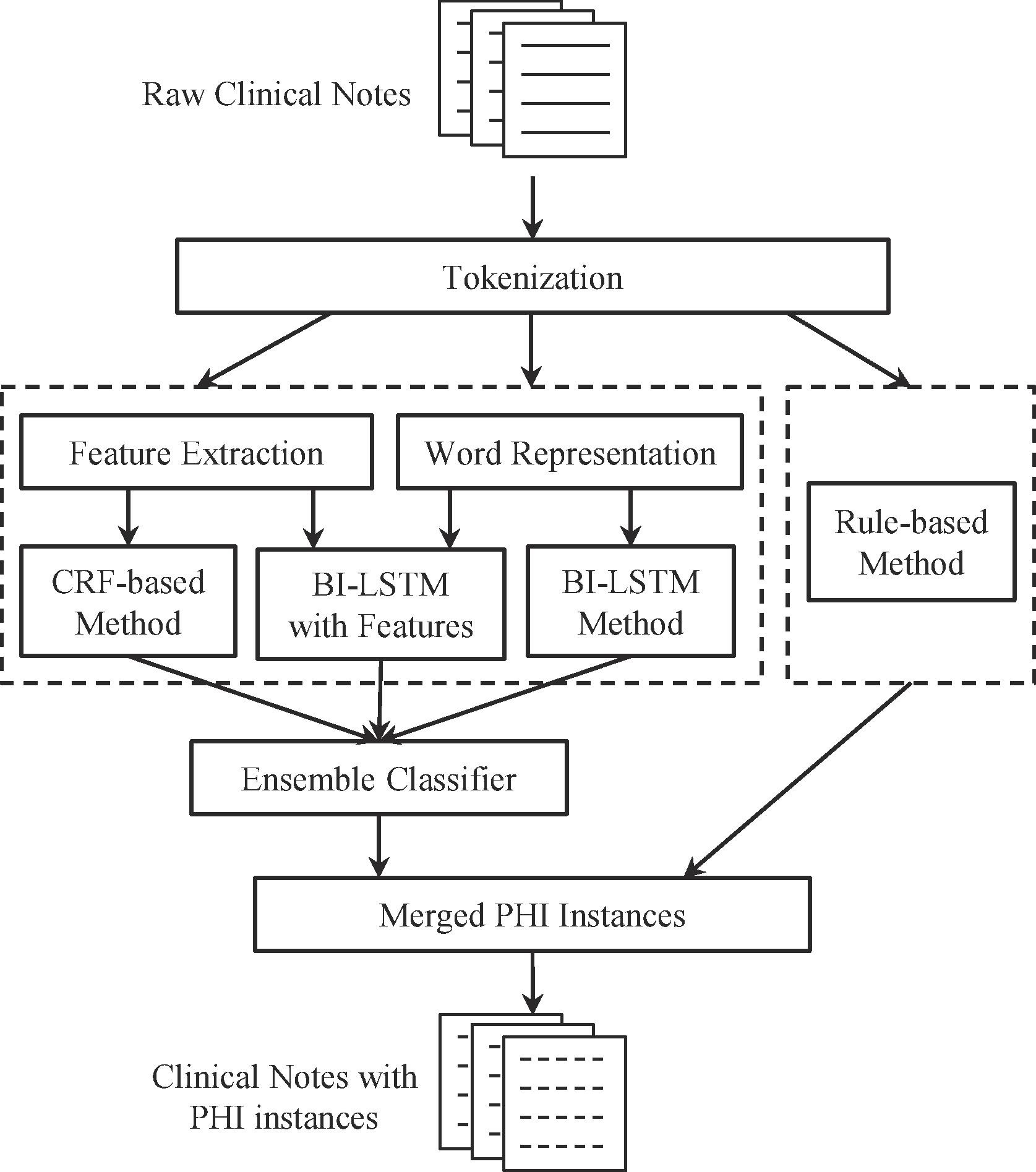
[1] Lee HJ, Wu Y, Zhang Y, Xu J, Xu H, Roberts K. A hybrid approach to automatic de-identification of psychiatric notes. Journal of biomedical informatics. 2017 Nov 1;75:S19-27. https://doi.org/10.1016/j.jbi.2017.06.006
What type of features can we build?
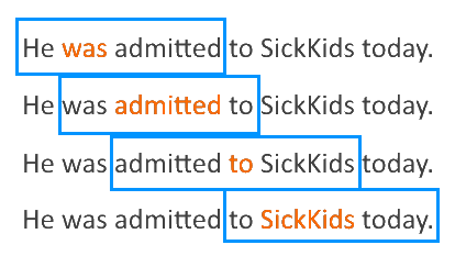
- Bag-of-words: unigrams, bigrams and trigrams of words within a window of [-2, 2].
Same as before, except we have switched from text classification to named entity recognition. That is, we are classifying words rather than the entire document, so we'll have a vector for each word, and there is a "window" around each word from which we'll extract data.
unigrams = ['Monday', 'Tuesday']
print(f'{"Entity":15s} -> [{", ".join(unigrams)}, ...]')
tokens = text.split(' ')
for i, token in enumerate(tokens):
    start, stop = max(i-2, 0), min(i+2+1, len(tokens))
    feature = [int(gram in tokens[start:stop]) for gram in unigrams]

    print(f'{token:15s} -> {", ".join(map(str, feature))}, ...')
Entity          -> [Monday, Tuesday, ...]
Alistair        -> 0, 0, ...
Johnson         -> 0, 0, ...
saw             -> 0, 0, ...
me              -> 1, 0, ...
last            -> 1, 0, ...
Monday          -> 1, 0, ...
the             -> 1, 0, ...
24th.           -> 1, 0, ...
- Bag-of-words: unigrams, bigrams and trigrams of words within a window of [-2, 2].
- Part-of-speech (POS) tags: unigrams, bigrams and trigrams of POS tags within a window of [−2, 2]. The Stanford POS Tagger [42] was used for POS tagging.
# spaCy has nifty functionality for understanding some of its outputs through spacy.explain
nlp = spacy.load('en_core_web_sm')
doc = nlp(text)
for token in doc:
    print(f'{token.text:15s}{token.tag_:5s}{spacy.explain(token.tag_)}')
Alistair       NNP  noun, proper singular
Johnson        NNP  noun, proper singular
saw            VBD  verb, past tense
me             PRP  pronoun, personal
last           JJ   adjective
Monday         NNP  noun, proper singular
the            DT   determiner
24th           NN   noun, singular or mass
.              .    punctuation mark, sentence closer
- Bag-of-words: unigrams, bigrams and trigrams of words within a window of [-2, 2].
- Part-of-speech (POS) tags: unigrams, bigrams and trigrams of POS tags within a window of [−2, 2]. The Stanford POS Tagger [42] was used for POS tagging.
- Word shapes: mapping any or consecutive uppercase character(s), lowercase character(s), digit(s) and other character(s) in current word to ’ A’, ’ a’, ’ #’ and ’ -’ respectively. For instance, the word shapes of “Hospital” are “Aaaaaaaa” and “Aa”.
word_shapes = []
for token in tokens:
    shape = ''
    for letter in token:
        if letter in 'ABCDEFGHIJKLMNOPQRSTUVWXYZ':
            shape += 'A'
        # note the bug in the below if statement :)
        elif letter in 'abcdefghijklmnopqrstuvwxtz':
            shape += 'a'
        elif letter in '0123456789':
            shape += '#'
        else:
            shape += '-'
    word_shapes.append(shape)
    print(f'{token:15s} {shape}')
Alistair        Aaaaaaaa
Johnson         Aaaaaaa
saw             aaa
me              aa
last            aaaa
Monday          Aaaaa-
the             aaa
24th.           ##aa-
Regular expressions (regex)
- Regex: match patterns in text
- Concise and powerful pattern matching language
- Supported by many computer languages, including SQL
- Challenges
- Brittle
- Hard to write, can get complex to be correct
- Hard to read
import re

text_modified = str(text)
print(text_modified)
Alistair Johnson saw me last Monday the 24th.
Replace capital letters with 'A'.
text_modified = re.sub('[A-Z]', 'A', text_modified)
print(text_modified)
Alistair Aohnson saw me last Aonday the 24th.
Replace lower case letters with 'a'.
text_modified = re.sub('[a-z]', 'a', text_modified)
print(text_modified)
Aaaaaaaa Aaaaaaa aaa aa aaaa Aaaaaa aaa 24aa.
Replace numbers with '#'.
text_modified = re.sub('[0-9]', '#', text_modified)
print(text_modified)
Aaaaaaaa Aaaaaaa aaa aa aaaa Aaaaaa aaa ##aa.
Replace the rest with '-'.
text_modified = re.sub('[^Aa# ]', '-', text_modified)
print(text_modified)
Aaaaaaaa Aaaaaaa aaa aa aaaa Aaaaaa aaa ##aa-
Features extracted in this one paper
- Bag-of-words: unigrams, bigrams and trigrams of words within a window of [-2, 2].
- Part-of-speech (POS) tags: unigrams, bigrams and trigrams of POS tags within a window of [−2, 2]. The Stanford POS Tagger [42] was used for POS tagging.
- Word shapes: mapping any or consecutive uppercase character(s), lowercase character(s), digit(s) and other character(s) in current word to ’ A’, ’ a’, ’ #’ and ’ -’ respectively. For instance, the word shapes of “Hospital” are “Aaaaaaaa” and “Aa”.
- Combinations of words and POS tags: combining current word with the unigrams, bigrams and trigrams of POS tags within a window of [−1, 1], i.e. w0p−1, w0p0, w0p1, w0p−1p0, w0p0p1, w0p−1p1, w0p−1p0p1, where w0, p−1, p0 and p1 denote current word, last, current and next POS tags respectively.
- Sentence information: number of words in current sentence, whether there is an end mark at the end of current sentence such as ’.’, ’?’ and ’!’, whether there is any bracket unmatched in current sentence.
- Affixes: prefixes and suffixes of length from 1 to 5.
- Orthographical features: whether the word is upper case, contains uppercase characters, contains punctuation marks, contains digits, etc.
- Section information: twenty-nine section headers (see the supplementary file) were collected manually such as “History of Present Illness”; we check which section current word belongs to.
- General NER information: the Stanford Named Entity Recognizer [43] was used to generate the NER tags of current word, include: person, date, organization, location, and number tags, etc.
Features extracted in this one paper
Happily, many NLP libraries have these features built in!
For example, named entity recognition.
displacy.render(doc, style='ent', jupyter=True)
# visualize the data with the sentence
alphabet = 'abcdefghijklmnopqrstuvwxyz'
X = prepare_data(sentences, alphabet=alphabet)
print(alphabet)
for i, sentence_vector in enumerate(X):
    print(''.join([str(c) for c in sentence_vector]), end=' ')
    print(sentences[i])
abcdefghijklmnopqrstuvwxyz
10011011100010100001000000 We had a good time.
10111011101101110010001000 This was a good-looking place.
10101100100111110101000100 A once in a lifetime experience.
01001000100100100100000000 Horrible.
00101101100111110111001110 One of the worst experiences of my life.
01001011100101000101111010 Everything went terribly, I'll never return.
Word embeddings
We have slowly improved the representation of our text
Then we moved to tokens, mostly word tokens.
# visualize the data with the sentence
alphabet = ['good', 'great', 'worst']
X = prepare_data(sentences, alphabet=alphabet)
print(' '.join([f'{c:10s}' for c in alphabet]))
for i, sentence_vector in enumerate(X):
    print(' '.join([f'{c:10d}' for c in sentence_vector]), end=' ')
    print(sentences[i])
good       great      worst
         1          0          0 We had a good time.
         1          0          0 This was a good-looking place.
         0          0          0 A once in a lifetime experience.
         0          0          0 Horrible.
         0          0          1 One of the worst experiences of my life.
         0          0          0 Everything went terribly, I'll never return.
Word embeddings
Intuitively, we know "good" and "great" are similar.
But the model has no mechanism for accounting for this. Anything it learns about good, it must also learn about great.
-> we don't share knowledge between "good" and "great"
Manually creating word embeddings
We could manually create these features - especially if we have a thesaurus! Synonyms for good (as a noun):
- that which is morally right; righteousness.
- "virtue", "righteousness", "virtuousness", "goodness", "morality", "ethicalness", "uprightness", "upstandingness", "integrity", "principle", "dignity", "rectitude", "rightness", "honesty", "truth", "truthfulness", "honor", "incorruptibility", "probity", "propriety", "worthiness", "worth", "merit", "irreproachableness", "blamelessness", "purity", "pureness", "lack of corruption", "justice", "justness", "fairness"
- benefit or advantage to someone or something.
- "benefit", "advantage", "profit", "gain", "interest", "welfare", "well-being", "enjoyment", "satisfaction", "comfort", "ease", "convenience", "help", "aid",
Manually creating word embeddings
But "good" has different meanings depending on its part of speech. When used as an adjective, we have many more options..
- having the qualities required for a particular role.
- "fine", "quality", "superior", "excellent", "superb", "outstanding", "magnificent", "exceptional", "marvelous", "wonderful", "first-rate", "first-class", "splendid", "ambrosial"
- skilled at doing or dealing with a specified thing.
- "capable", "able", "proficient", "adept", "adroit", "accomplished", "seasoned", "skillful", "skilled", "gifted", "talented", "masterly", "virtuoso", "expert", "knowledgeable", "qualified", "trained", "great", "mean", "wicked", "deadly", "nifty", "crack", "super", "ace", "wizard", "magic"
- useful, advantageous, or beneficial in effect.
- "wholesome", "health-giving", "healthful", "healthy", "nourishing", "nutritious", "nutritional", "strengthening", "beneficial", "salubrious", "salutary"
- appropriate to a particular purpose.
- "convenient", "suitable", "appropriate", "fitting", "fit", "suited", "agreeable", "opportune", "timely", "well timed", "favorable", "advantageous", "expedient", "felicitous", "propitious", "auspicious", "happy", "providential", "commodious", "seasonable"
- possessing or displaying moral virtue.
- "virtuous", "righteous", "moral", "morally correct", "ethical", "upright", "upstanding", "high-minded", "right-minded", "right-thinking", "principled", "exemplary", "clean", "law-abiding", "lawful", "irreproachable", "blameless", "guiltless", "unimpeachable", "just", "honest", "honorable", "unbribable", "incorruptible", "anticorruption", "scrupulous", "reputable", "decent", "respectable", "noble", "lofty", "elevated", "worthy", "trustworthy", "meritorious", "praiseworthy", "commendable", "admirable", "laudable", "pure", "pure as the driven snow", "whiter than white", "sinless", "saintly", "saintlike", "godly", "angelic", "squeaky clean"
- showing kindness.
- "kind", "kindly", "kindhearted", "good-hearted", "friendly", "obliging", "generous", "charitable", "magnanimous", "gracious", "sympathetic", "benevolent", "benign", "altruistic", "unselfish", "selfless"
- obedient to rules or conventions.
- "well behaved", "obedient", "dutiful", "well mannered", "well brought up", "polite", "civil", "courteous", "respectful", "deferential", "manageable", "compliant", "acquiescent", "tractable", "malleable", "right", "correct", "proper", "decorous", "seemly", "appropriate", "fitting", "apt", "suitable", "convenient", "expedient", "favorable", "auspicious", "propitious", "opportune", "felicitous", "timely", "well judged", "well timed", "meet", "seasonable"
- giving pleasure; enjoyable or satisfying.
- "enjoyable", "pleasant", "agreeable", "pleasing", "pleasurable", "delightful", "great", "nice", "lovely", "amusing", "diverting", "jolly", "merry", "lively", "festive", "cheerful", "convivial", "congenial", "sociable", "super", "fantastic", "fabulous", "fab", "terrific", "glorious", "grand", "magic", "out of this world", "cool", "brilliant", "brill", "smashing", "peachy", "neat", "ducky", "beaut", "bonzer", "capital", "wizard", "corking", "spiffing", "ripping", "top-hole", "topping", "champion", "beezer", "swell", "frabjous"
- (of clothes) smart and suitable for formal wear.
- "best", "finest", "newest", "nice", "nicest", "smart", "smartest", "special", "party", "Sunday", "formal", "dressy", "Opposite", "casual", "scruffy",
Manually creating word embeddings
And that's not all! The meaning of "good" depends on its context.
- Very good
- "admirable", "brilliant", "exceptional", "fantastic"
- Be good
- "manage", "comport oneself", "act with decorum", "be civil"
We have one word and 13 features already - and we haven't even been exhaustive. We need a new approach. Wouldn't it be great if we could instead learn these features, rather than manually engineer them?
Distributional hypothesis
- Does language have a distributional structure? [1]
structure:
A set of phonemes or a set of data is structured in respect to some feature, to the extent that we can form in terms of that feature some organized system of statements which describes the members of the set and their interrelations (at least up to some limit of complexity).
distributional:
The distribution of an element will be understood as the sum of all its environments. An environment of an element A is an existing array of its co-occurrents, i.e. the other elements, each in a particular position, with which A occurs to yield an utterance.
-> you're known by the company you keep
[1] Harris ZS. Distributional structure. Word. 1954 Aug 1;10(2-3):146-62. PDF.
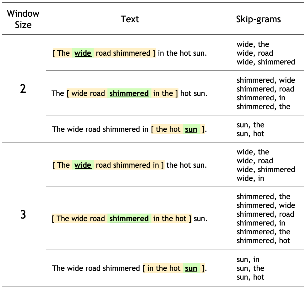
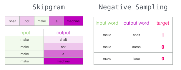
word2vec
Learn these features, rather than manually create them.
- Take a whole bunch of text
- Try to predict a word's context form the word itself ("skip-grams")
- Use the model's representation of words (tokens)
nlp = spacy.load("en_core_web_sm")
text = 'good great capable wholesome convenient virtuous kind virtue'
tokens = nlp(text)

vectors = []

for token in tokens:
    print(f'{token.text:10s}{token.has_vector} {token.vector_norm} {[f"{t:1.2f}" for t in token.vector[:5]]} ...')
    vectors.append(token.vector)

vectors = np.vstack(vectors)
good      True 6.793087005615234 ['-0.90', '-0.70', '1.23', '-0.03', '-0.53'] ...
great     True 7.209250450134277 ['-0.28', '-0.11', '0.94', '-0.10', '-0.23'] ...
capable   True 7.762300491333008 ['-0.02', '-0.54', '-0.41', '-0.69', '0.55'] ...
wholesome True 7.631638526916504 ['-1.28', '0.79', '1.74', '-0.82', '-0.58'] ...
convenientTrue 7.83421516418457 ['-0.41', '-0.02', '0.56', '-0.00', '0.42'] ...
virtuous  True 7.114853858947754 ['0.65', '0.29', '0.47', '-0.16', '0.17'] ...
kind      True 7.497698783874512 ['0.33', '-0.39', '1.95', '-0.12', '-0.12'] ...
virtue    True 7.287103652954102 ['1.07', '0.35', '0.67', '0.13', '-0.03'] ...
import seaborn as sns
import matplotlib.pyplot as plt

plt.figure(figsize=[12, 8])
sns.heatmap(vectors, yticklabels=[token.text for token in tokens])
plt.show()

Remember that the embedding dimension (x-axis) has no intrinsic order - so we can re-order it to make it easier to see relations
from scipy.spatial.distance import pdist, cdist
from seriate import seriate
reorder_dims = seriate(pdist(vectors.T, metric='cosine'))
plt.figure(figsize=[12, 8])
sns.heatmap(vectors[:, reorder_dims], yticklabels=[token.text for token in tokens])
plt.gca().axes.xaxis.set_ticklabels([])
plt.show()

nlp = spacy.load("en_core_web_md")
X_train_vectors = []
X_test_vectors = []
# only enable the vectorize step to speed up processing
with nlp.select_pipes(enable="tok2vec"):
    for text in tqdm(X_train, total=X_train.shape[0]):
        doc = nlp(str(text))
        # doc.vector contains the average of all token vectors
        X_train_vectors.append(doc.vector)

    for text in tqdm(X_test, total=X_test.shape[0]):
        doc = nlp(str(text))
        X_test_vectors.append(doc.vector)

X_train_vectors = np.vstack(X_train_vectors)
X_test_vectors = np.vstack(X_test_vectors)
pipe = Pipeline([('classifier', tree.DecisionTreeClassifier(max_depth=3))])

pred = train_pipe_and_predict(pipe, X_train_vectors, y_train, X_test_vectors)

print_results(y_test, pred)
Building model.
Getting test predictions.
Accuracy: 63.2%
Precision: 66.1%
Recall: 54.1%
classifier = pipe.named_steps['classifier']

# blue = positive, orange = negative
graph = create_graph(classifier)
Image(graph.create_png())

from sklearn.decomposition import PCA
from sklearn.manifold import TSNE

# get 3 principle components
pca = PCA(n_components=2)
pca_result = pca.fit_transform(X_train_vectors)

# TSNE
tsne = TSNE(n_components=2, verbose=1, perplexity=40, n_iter=300)
tsne_results = tsne.fit_transform(pca_result)


plt.figure(figsize=(16,10))
sns.scatterplot(
    x=tsne_results[:,0], y=tsne_results[:,1],
    hue=y_train,
    palette=sns.color_palette("bright", 2),
    legend="full",
    alpha=0.3
)
plt.show()
[t-SNE] Computing 121 nearest neighbors...
[t-SNE] Indexed 2222 samples in 0.002s...
[t-SNE] Computed neighbors for 2222 samples in 0.086s...
[t-SNE] Computed conditional probabilities for sample 1000 / 2222
[t-SNE] Computed conditional probabilities for sample 2000 / 2222
[t-SNE] Computed conditional probabilities for sample 2222 / 2222
[t-SNE] Mean sigma: 0.033471
[t-SNE] KL divergence after 250 iterations with early exaggeration: 61.015236
[t-SNE] KL divergence after 300 iterations: 0.792019

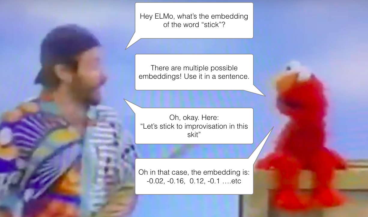
We haven't handled context yet!
We've learned what the word "good" means, but the meaning does not change between "be good" and "very good". Easier to think about this for homonyms (specifically homographs):
- The bank robber got away.
- The river bank is slippery.
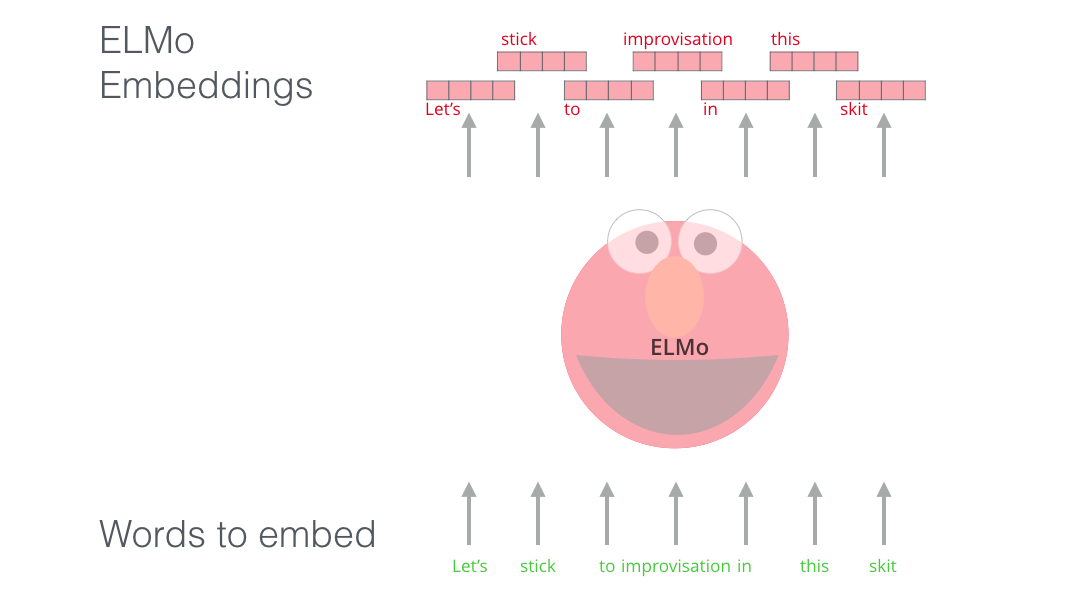
Sesame street to the rescue - Illustrated BERT by Jay Alammar
![]()
Sesame street to the rescue - Illustrated BERT by Jay Alammar
Sesame street to the rescue - Illustrated BERT by Jay Alammar
Experimenting with BERT
One good way is to experiment with Google's tutorial:
What libraries do people use?
spaCy pipeline

- Tokenize: split text into individual meaningful units
- Pre-process: remove stop words, remove punctuation
- Stemming: remove the suffix of words to merge similar words together
- Lemmatize: use a lexicon to merge similar words together
- Extract features: do whatever you think makes sense!
Further reading
- http://web.stanford.edu/class/cs224n/
- https://github.com/fastai/course-nlp
- http://norvig.com/ngrams/
- The shallowness of Google translate - we still have some way to go!